On Device Training

This section shows you a simple application to test on device training capabilities of edge devices using the dAIEdge-VLab Python API.

What does this application do ?

In this application example, we will prepare a model with Tensorflow, prepare a train dataset, prepare a validation dataset and train the model on a remote device. Finally, we will analyze the results given by the remote device.

The following diagram shows the pipeline of this application :

  sequenceDiagram
    participant User
    participant dAIEdge-VLab
    participant Target
    User->>User: Prepare Datasets
    User->>User: Prepare Model for training
    User->>dAIEdge-VLab: Model, Datasets, Config, Target, Runtime
    dAIEdge-VLab->>Target: Model, Datasets, Config
    Target->>Target: Perfom the training on device
    Target->>dAIEdge-VLab: report, logs, trained model
    dAIEdge-VLab->>User: report, logs, trained model
    User->>User: Print loss evolution
    User->>User: Test trained model
    User->>User: Compute accuracy metrics

Main actions :

Prepare the datasets on the user end
Pre-train the model on the user end (optional)
Setup the model for on device training
Send the model and datasets to the dAIEdge-VLab
Train the model on the remote device
Retrive the trained model from the remote device
Analyze the resutls

What problem will be solved ?

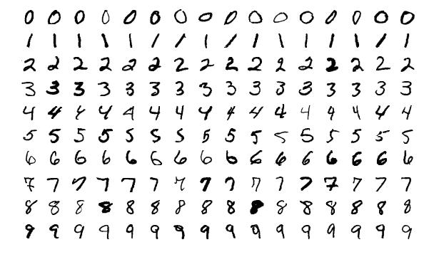
In this simple application, we will train a model to recogize numbers from an image. We will use the MNIST dataset as based for the training and testing of the model. The image bellow illustrates the kind of images that compose the dataset. Our model will simply take an image as input and output a prediction of the number that was on the image.

The output of the model will be one hot encoded. This means that we will have one output node per class we want to detect. In this case this is 10 classes as they are 10 numbers from 0 to 9. Knowing the input and ouput shape is important for the preparation of the dataset we will provide to the dAIEdge-VLab.

Prepare the envionement

For this application example you will need to have a Python 3.8 environement wiht tensoflow 2.8.0, numpy, matplotlib and daiedge-vlab installed. Use the step-by-step user guide to install and setup the daiedge-vlab package. Use the following requirements.txt file to install the other depedencies:

pip install -r requirements.txt

Implement Application

The following section shows a simple but complete application to prepare a model for on device training, train it on the MNIST dataset and validate the model on a remote target.

Define the model architecture

To train a simple model that will recogize the number on an image we can use a simple but effective neural network structure. The model will be composed of :

The input layer made of 28x28x1 nodes
A Conv2D (32 filters, 3x3 kernel, ReLU activation) layer
A MaxPooling2D (2x2 pool size) layer
A Conv2D (64 filters, 3x3 kernel, ReLU activation)
A axPooling2D (2x2 pool size) layer
A Flatten layer : Converts 2D feature maps into a 1D vector for the dense layer.
A Dense (128 neurons, ReLU activation) layer
A Dense (10 neurons, softmax activation) layer : The output layer

Prepare the different datasets

From the MNIST dataset we create 3 sub-datasets :

A train dataset (used to train the model)
A test dataset (used to test the model)

The following code defines a function to prepare the datasets, preprocess them, and save them in binary format. This function will be used later in the application to load the datasets for training and testing. Note the different names of the binary files that will be created. These names will be setup in the config.yaml file used to configure the on device training experiment.

from daiedge_vlab import dAIEdgeVLabAPI, OnDeviceTrainingConfig
import tensorflow as tf
import numpy as np
import matplotlib.pyplot as plt

############################################
# Configuration
############################################

SETUP_FILE = "setup.yaml"

TARGET = 'rpi5'
RUNTIME = 'tflite'
MODEL = 'model.tflite'

TRAIN_NB_SAMPLES = 10000
TEST_NB_SAMPLES = 2000

RESULT_DIR = "./results"

############################################
# Step 1: Load, Preprocess MNIST, and Save Data
############################################

def prepare_datasets():
    # Load MNIST dataset.
    (x_train, y_train), (x_test, y_test) = tf.keras.datasets.mnist.load_data()

    # Preprocess: Convert images to float32, normalize to [0,1], and add channel dimension.
    x_train = (x_train.astype(np.float32) / 255.0)[..., np.newaxis]
    x_test  = (x_test.astype(np.float32) / 255.0)[..., np.newaxis]

    # Reduce the size of the dataset for faster training (optional).
    x_train = x_train[:TRAIN_NB_SAMPLES]  
    y_train = y_train[:TRAIN_NB_SAMPLES]
    x_test  = x_test[:TEST_NB_SAMPLES]    
    y_test  = y_test[:TEST_NB_SAMPLES]

    # Preprocess labels.
    y_train = y_train.astype(np.int32)
    y_test = y_test.astype(np.int32)

    # Save preprocessed data as binary files.
    x_train.tofile("mnist_train_input.bin")
    y_train.tofile("mnist_train_target.bin")
    x_test.tofile("mnist_test_input.bin")
    y_test.tofile("mnist_test_target.bin")

    print(len(x_train), len(y_train), len(x_test), len(y_test))
    print("Preprocessed train/test data saved as .bin files.")
    return (x_train, y_train), (x_test, y_test)

Define the model architecture

The following code defines a simple Keras model that will be used for on device training. The model is a Convolutional Neural Network (CNN) suitable for image classification tasks like MNIST digit recognition.

############################################
# Step 2: Define a Simple Keras Model.
############################################
def create_model():
    inputs = tf.keras.Input(shape=(28, 28, 1), name="input")
    x = tf.keras.layers.Conv2D(32, 3, activation="relu")(inputs)
    x = tf.keras.layers.MaxPooling2D()(x)
    x = tf.keras.layers.Conv2D(64, 3, activation="relu")(x)
    x = tf.keras.layers.MaxPooling2D()(x)
    x = tf.keras.layers.Flatten()(x)
    x = tf.keras.layers.Dense(128, activation="relu")(x)
    outputs = tf.keras.layers.Dense(10, activation="softmax", name="output")(x)
    return tf.keras.Model(inputs, outputs)

Define the signature for the training

For the on device training, we need to define the training and inference signatures (and a save signature). The training signature will be used to perform one training step on the remote target. The inference signature will be used to perform inference on the remote target. The save signature will be used to save the model on the remote target. The following code defines these signatures using TensorFlow’s tf.function decorator. This allows us to specify the input signatures for the training and inference functions, which is necessary for the dAIEdge-VLab to understand how to interact with the model during on device training.

############################################
# Step 3: Define Custom Training and Inference Signatures.
############################################
# Training signature: performs one training step.
@tf.function(input_signature=[
    tf.TensorSpec([None, 28, 28, 1], tf.float32, name="x"),
    tf.TensorSpec([None], tf.int32, name="y")
])
def train_step(x, y):
    with tf.GradientTape() as tape:
        predictions = model(x, training=True)
        loss = tf.keras.losses.sparse_categorical_crossentropy(y, predictions)
        loss = tf.reduce_mean(loss)
    gradients = tape.gradient(loss, model.trainable_variables)
    model.optimizer.apply_gradients(zip(gradients, model.trainable_variables))
    return {"loss": loss}

# Inference signature: performs a forward pass (inference).
@tf.function(input_signature=[
    tf.TensorSpec([None, 28, 28, 1], tf.float32, name="input")
])
def inference(x):
    predictions = model(x, training=False)
    return {"output": predictions}

# Save signature: receives a checkpoint path as input and returns a simple status.
@tf.function(input_signature=[tf.TensorSpec(shape=[], dtype=tf.string)])
def save(checkpoint_path):
    tensor_names = [weight.name for weight in model.weights]
    tensors_to_save = [weight.read_value() for weight in model.weights]
    tf.raw_ops.Save(
        filename=checkpoint_path, tensor_names=tensor_names,
        data=tensors_to_save, name='save')
    return {"status": tf.constant("saved")}

Define the restore function given a checkpoint path

The restore function is used to restore the model weights from a checkpoint file. This is useful when we want to load a previously trained model on the remote target. The function takes a checkpoint path as input and the model architecture. It restores the model weights from that checkpoint. The function uses TensorFlow’s tf.raw_ops.RestoreV2 operation to read the weights from the checkpoint file and assign them to the model weights.

############################################
# Step 3: Define a Function to Restore Checkpoint Variables.
############################################
def restore_raw_checkpoint(model, ckpt_prefix):
    """Load variables saved with tf.raw_ops.Save into *model*."""
    var_names  = [w.name for w in model.weights]  
    dtypes     = [w.dtype for w in model.weights]

    print(f"Restoring weights from {var_names}...")

    # Restore every tensor in one call
    restored = tf.raw_ops.RestoreV2(
        prefix            = ckpt_prefix,
        tensor_names      = var_names,
        shape_and_slices  = [""] * len(var_names),
        dtypes            = dtypes
    )

    # Copy restored values back into the Keras weights
    for tensor, weight in zip(restored, model.weights):
        weight.assign(tensor)

    print(f"OK: Weights restored from {ckpt_prefix}")

Build the pipeline for on device training

Now that we have the model architecture and the signatures defined, we can build the pipeline for on device training. This pipeline will include the following steps:

Prepare the datasets.
Create the model.
Compile the model.
Define the training and inference signatures.
Save the model in a format compatible with on device training.
Upload the model and datasets to the dAIEdge-VLab.
Restore the model weights from the recieived checkpoint file on the remote target.
Plot the training loss evolution.

Start by creating the datasets and the model, then compile the model. The model will be compiled with the Adam optimizer and the sparse categorical crossentropy loss function. You may want to pre-train the model on the user end before sending it to the remote target. This is optional and can be done by uncommenting the model.fit line. If you do not pre-train the model, the model will be trained on the remote target from scratch. If you pre-train the model, you can choose to make all layers trainable or only the last layer. In this example, we will make all layers trainable. We finally save the model with both training and inference signatures. The model will be saved in a directory named mnist_model.

# Load and preprocess the MNIST dataset.
(x_train, y_train), (x_test, y_test) = prepare_datasets()

# Create the nmodel 
model = create_model()

model.compile(optimizer="adam",
            loss="sparse_categorical_crossentropy",
            metrics=["accuracy"])

# Optional - pre-train the model (adjust epochs as needed).
# model.fit(x_train, y_train, epochs=1, validation_data=(x_test, y_test))

# Make all layers trainable.
model.trainable = True   
# Alternatively, you can set specific layers to be trainable.
# For example, if you want to train only the last layer:
#for layer in model.layers:
#    layer.trainable = False
#model.layers[-1].trainable = Trueainable = True  

############################################
# Step 4: Save the Model as a SavedModel with Both Signatures.
############################################
# Both signatures are exported:
# - "train" for on-device training,
# - "serving_default" for inference.
model.save("mnist_model", signatures={
    "train": train_step.get_concrete_function(),
    "serving_default": inference.get_concrete_function(),
    "save": save.get_concrete_function()
})
print("SavedModel with training and inference signatures saved to 'mnist_model'.")

Once the model is saved, we can convert it to a format compatible with on device training. In this case, we will convert it to a TensorFlow Lite model. The conversion is done using the tf.lite.TFLiteConverter class. The converted model will be saved in a file named model.tflite. We also need to make sure the model is compatible with on device training.

############################################
# Step 5: Convert the SavedModel to a TFLite Model for On‑Device Training.
############################################
converter = tf.lite.TFLiteConverter.from_saved_model("mnist_model")
# Retain mutable (resource) variables required for training.
converter.experimental_enable_resource_variables = True
# Optionally support extra TF ops.
converter.target_spec.supported_ops = [
    tf.lite.OpsSet.TFLITE_BUILTINS,
    tf.lite.OpsSet.SELECT_TF_OPS
]
tflite_model = converter.convert()

# Save the TFLite model.
with open(MODEL, "wb") as f:
    f.write(tflite_model)
print("TFLite model with on-device training support saved as 'model.tflite'.")

We are now almost ready to send the model and datasets to the dAIEdge-VLab. We need to create a configuration file that will be used to configure the on device training experiment. This configuration file will be named config.json and will contain the following information:

config.json

{
    "learning_parameters" : {
      "batch_size": 32,
      "epochs": 10,
      "loss_function": "sparse_categorical_crossentropy"
    },
    "input": {
      "name": "input",
      "shape": [28, 28, 1],
      "dtype": "float32",
      "train_file": "mnist_train_input.bin",
      "test_file": "mnist_test_input.bin"
    },
    "output": {
      "name": "output",
      "shape": [],
      "dtype": "int32",
      "train_file": "mnist_train_target.bin",
      "test_file": "mnist_test_target.bin"
    }
}

This json file contains the learning parameters, the input and output shapes, the data types, and the names of the train and test files. The input shape is [28, 28, 1] because we are working with grayscale images of size 28x28. The output shape is [] because we are using sparse categorical crossentropy loss function which expects a single integer label per sample.

Once the config.json file is created, we can create OnDeviceTrainingConfig object that will load the configuration file. This object will be used to start the on device training experiment.

############################################
# Step 6: Upload the Model and Start the Benchmark.
############################################
# Log in to the dAIEdge VLab API.
api = dAIEdgeVLabAPI(SETUP_FILE)

# Parse the configuration file for on-device training.
# Make sure to adjust the path to your config file.
config = OnDeviceTrainingConfig("./config.json")

# Start the benchmark with the specified target, runtime, dataset and model.
id = api.startOdtBenchmark(
    TARGET,
    RUNTIME,
    MODEL,
    config
)

# Wait for the benchmark to finish and save the results.
print(f"Benchmark started with ID: {id}")

r = api.waitBenchmarkResult(id, save_path=RESULT_DIR, verbose=True)
print("Benchmark finished:", r)

Analyze the results

Once the benchmark is finished, we can analyze the results. The report contains the evolution of the training loss and the test loss over the different epochs. It can be plotted using the matplotlib library. The following code will plot the training and test loss evolution over the epochs. It will also train the train time per epoch and the average training time per epoch. The plot will be saved in a file named training_metrics.png. All the available metrics in the report can be found here : Odt Report keys.

############################################
# Step 7: Plot the metrics gathered during the on-device training.
############################################

# data lists (epoch, value)
train_loss = [(l["epoch_index"], l["loss"])  for l in r["report"]["loss_train"]["epochs"]]
test_loss  = [(l["epoch_index"], l["loss"])  for l in r["report"]["loss_test"]["epochs"]]
train_time = [(l["epoch_index"], l["time"])  for l in r["report"]["loss_train"]["epochs"]]

# unpack data lists
# epochs, tr_loss_vals, te_loss_vals, tr_time_vals
epochs,  tr_loss_vals = zip(*train_loss)
_,       te_loss_vals = zip(*test_loss)
_,       tr_time_vals = zip(*train_time)
tr_avrge_time = np.mean(tr_time_vals)

# side-by-side figure
fig, axes = plt.subplots(nrows=1, ncols=2, figsize=(12, 5), sharex=True)

# left panel - losses
axes[0].plot(epochs, tr_loss_vals, label="Train Loss")
axes[0].plot(epochs, te_loss_vals, label="Test Loss")
axes[0].set_xlabel("Epoch")
axes[0].set_ylabel("Loss")
axes[0].set_title("Loss over Epochs")
axes[0].legend()

# right panel - time per epoch
axes[1].plot(epochs, tr_time_vals, label="Train Time", color="orange")
axes[1].axhline(tr_avrge_time, color="red", linestyle="--", label="Avg Time")
axes[1].set_xlabel("Epoch")
axes[1].set_ylabel("Time (s)")
axes[1].set_title("Training Time per Epoch")
axes[1].legend()

fig.tight_layout()
fig.savefig("training_metrics.png", dpi=150)

The plot should look like this: Training Loss Over Epochs

Retrieve the trained model and test it

Finally, it is possible the retrive the trained model from the remote target and test it on the user end. The .ckpt file is already in the results directory. We can use the restore_raw_checkpoint function to restore the model weights from the checkpoint file. The restored model can then be used to perform inference on the test dataset. The name of the checkpoint file is given by the result of the benchmark in r["model_output"]. The following code will restore the model weights from the checkpoint file and perform inference on the test dataset. It will also compute the accuracy of the model on the test dataset.

############################################
# Step 8: Restore the Model and Evaluate on Test Set.
############################################

# Locate the model output in the results.
model_res = r["model_output"]
print(f"Model output: {model_res}")
ckpt_path = f"{RESULT_DIR}/{model_res}"  
assert tf.io.gfile.exists(ckpt_path), "Checkpoint not found!"

# Restore the model
tf.keras.backend.clear_session()

# Recreate a fresh model instance 
model = create_model()
model.compile(optimizer="adam",
            loss="sparse_categorical_crossentropy",
            metrics=["accuracy"])

# Restore the weights from the checkpoint.
restore_raw_checkpoint(model, ckpt_path)

# Evaluate the model on the test set.
loss, acc = model.evaluate(x_test, y_test, verbose=1)
print(f"loss: {loss:.4f}")    
print(f"Accuracy after on-device fine-tuning: {acc:.4f}")

# Save the updated model as a TFLite model with the new weights.
converter = tf.lite.TFLiteConverter.from_keras_model(model)
lite_trained = converter.convert()
with open("model_trained.tflite", "wb") as f:
    f.write(lite_trained)
print("Wrote model_trained.tflite with updated weights.")

You should see the accuracy of the model on the test dataset printed in the console like this:

OK: Weights restored from ./results/6676_trained_model.ckpt
63/63 [==============================] - 0s 1ms/step - loss: 0.0831 - accuracy: 0.9765
loss: 0.0831
Accuracy after on-device fine-tuning: 0.9765
...

You can download the enrire code of this application example here: odt_example.py.

Benchmark with hardware in the loop